Summary
Particle reconstruction in the ATLAS detector is the practice of associating calorimeter and tracker signals particle and determining which particles caused them, with how much energy, and through what process. One crucial step in reconstruction is cell segmentation where we determine which calorimeter signals belong to which tracks from the inner tracker. Current methods to perform segmentation rely on algorithms that grow with quadratic complexity, posing a challenge for segmentation after the High-Luminosity LHC (HL-LHC) upgrade, which promises a significant increase in the number of collisions per event and, therefore, the complexity of each event. Working under Dr. Max Swiatlowski, I am applying PointNet and other machine learning approaches to cell segmentation in the ATLAS calorimeter.
This summer, I have been fortunate enough to receive the Erich Vogt First Year Summer Research Experience Award (FYSRE), giving me the opportunity to work at TRIUMF, Canada’s Particle Accelerator Centre.
Note that this summary of my first month’s work is aimed at a semi-technical audience. If you have questions about the specifics or about any of the terms I use, please feel free to reach out to me.
Understanding the Problem
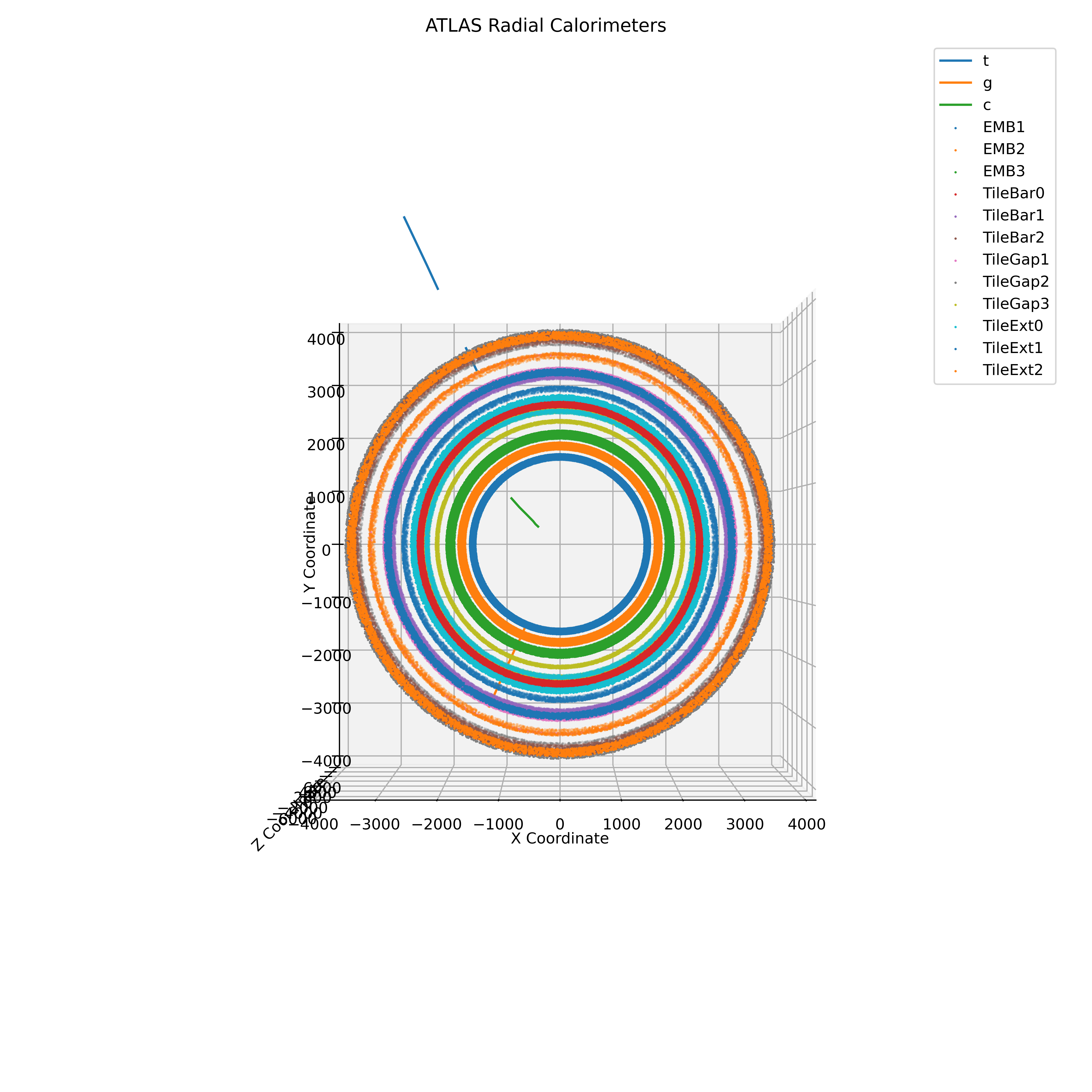
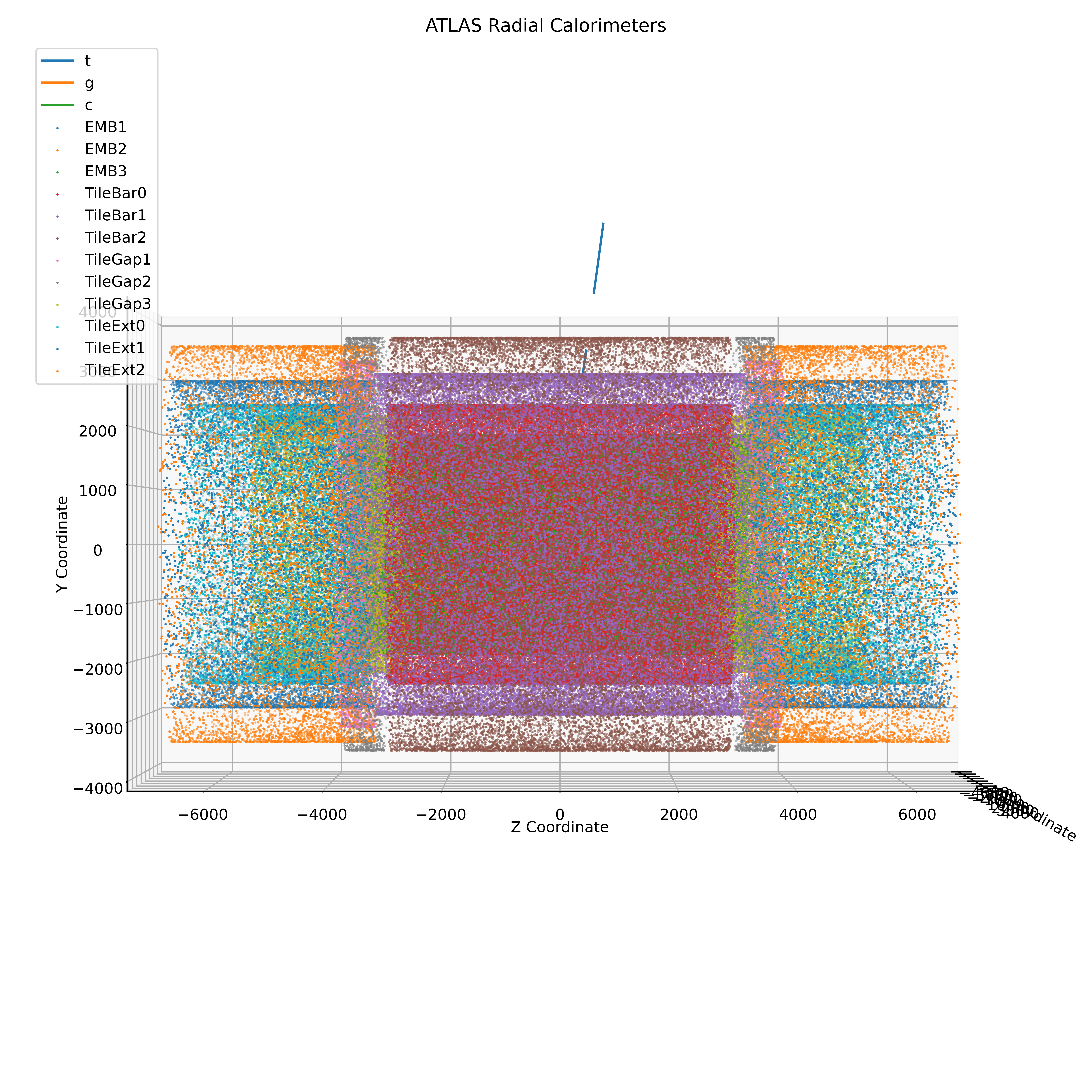
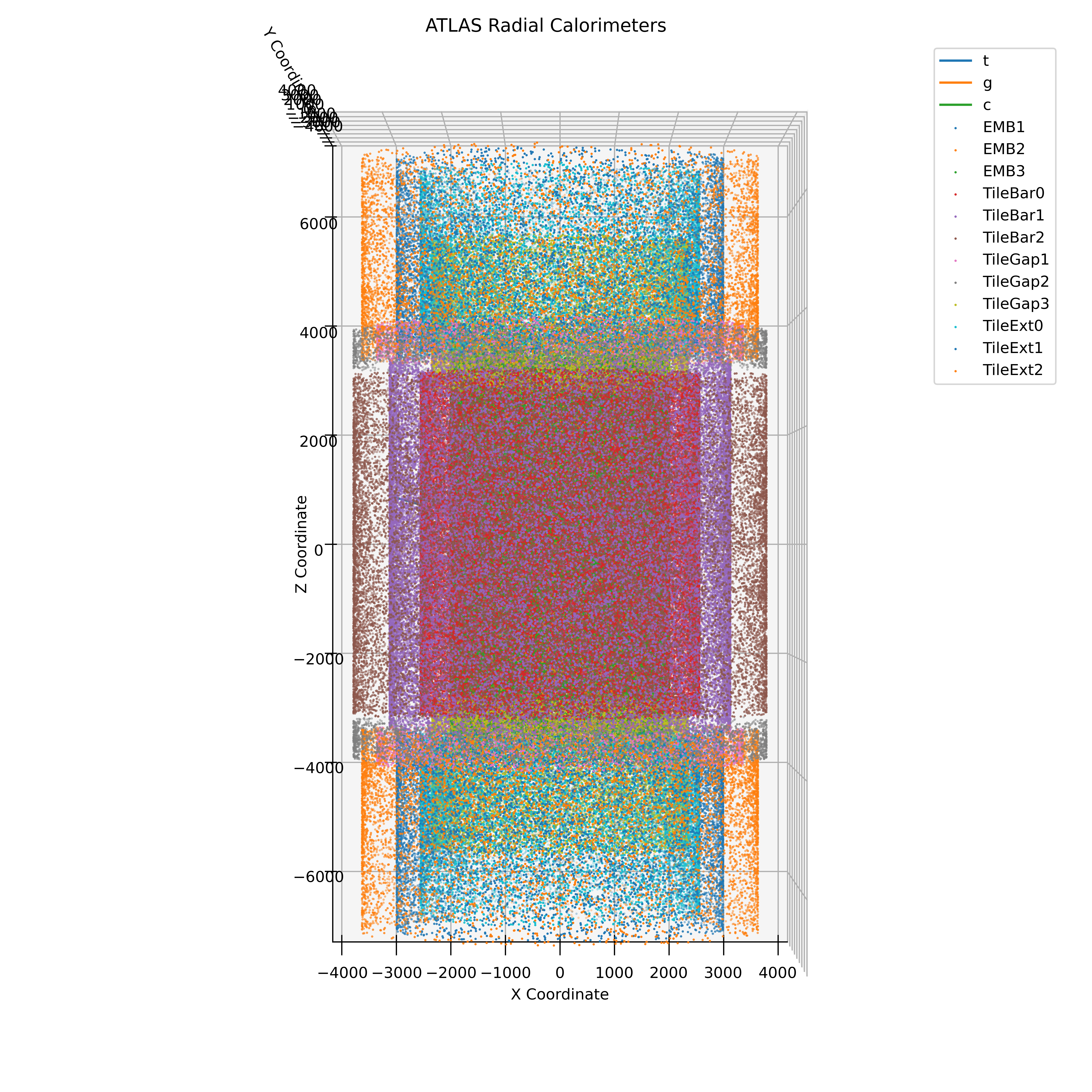
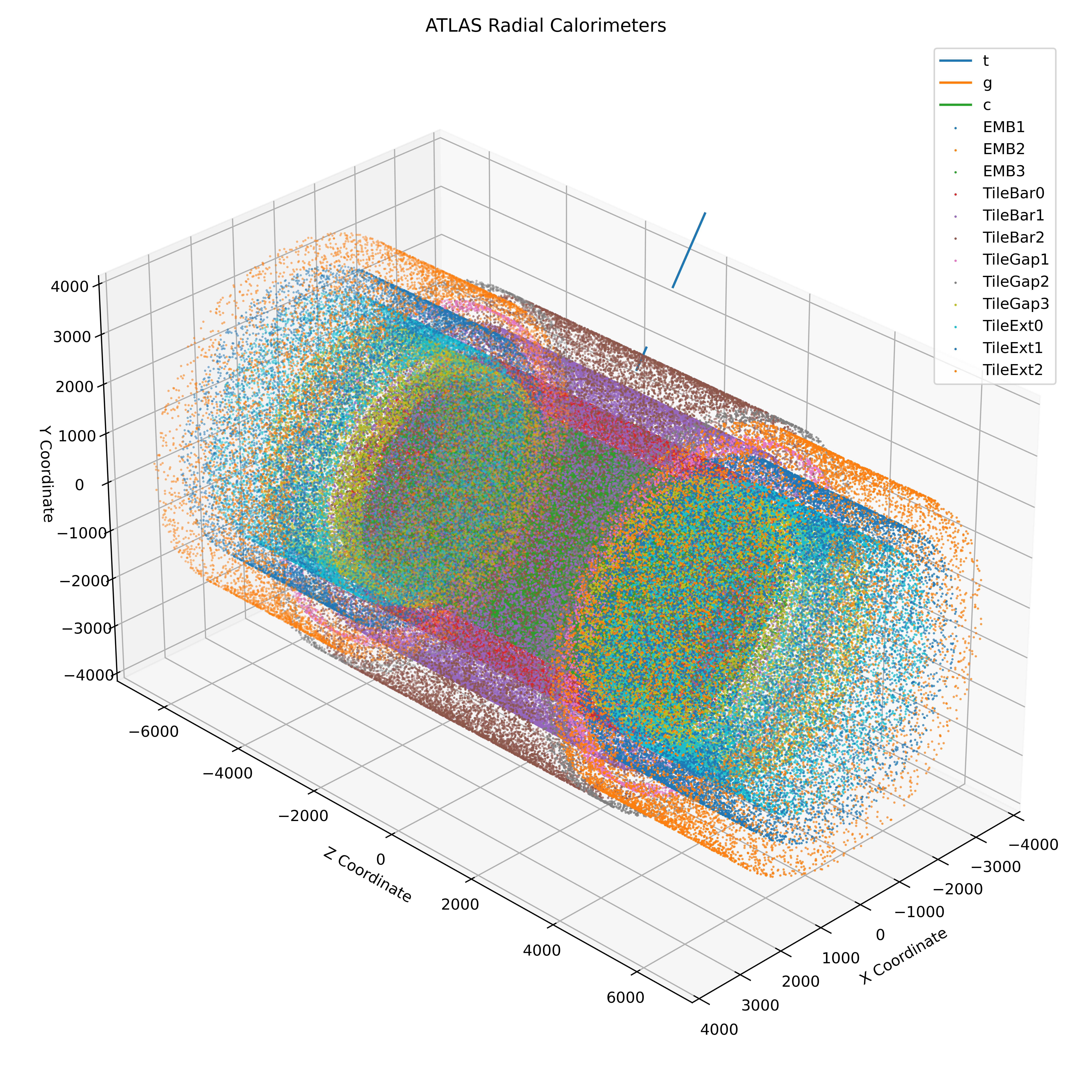
There are two primary types of detectors present in ATLAS. First, the inner trackers use silicon detectors to measure the path of charged particles. Thanks to the magnetic field in the LHC, the curvature of the particle’s path can be used to determine the momentum of particles in the tracker; however, not their energy. After passing through the inner tracker, particles enter the second type of detector, the calorimeter. The ATLAS calorimeter comprises many layers, including both the electromagnetic and hadronic calorimeters, which can absorb and read out the energy of (most) particles that pass through them.
|
|
|---|---|
|
|
One of the challenges of the ATLAS calorimeter is that relating the energy deposits in the calorimeter layers to tracks in the inner detector is non-trivial for several reasons.
- Some particles do not leave tracks in the inner tracker, such as photons and neutral hadrons, which will not ionize the silicon detectors.
- Some particles will leave tracks in the inner tracker but not in the calorimeter, like muons, which are so massive that they pass through the calorimeter without interacting with it.
- Lastly, and most importantly, because the LHC collides bunches containing millions of protons, there are often multiple closely spaced particle tracks. This effect, often termed pileup, can make it computationally expensive to relate calorimeter hits to tracks in the inner detector. As the LHC is upgraded to the HL-LHC (High-Luminosity LHC), the number of collisions per event will increase drastically, making this problem even more challenging.
Developing the Model
PointNet
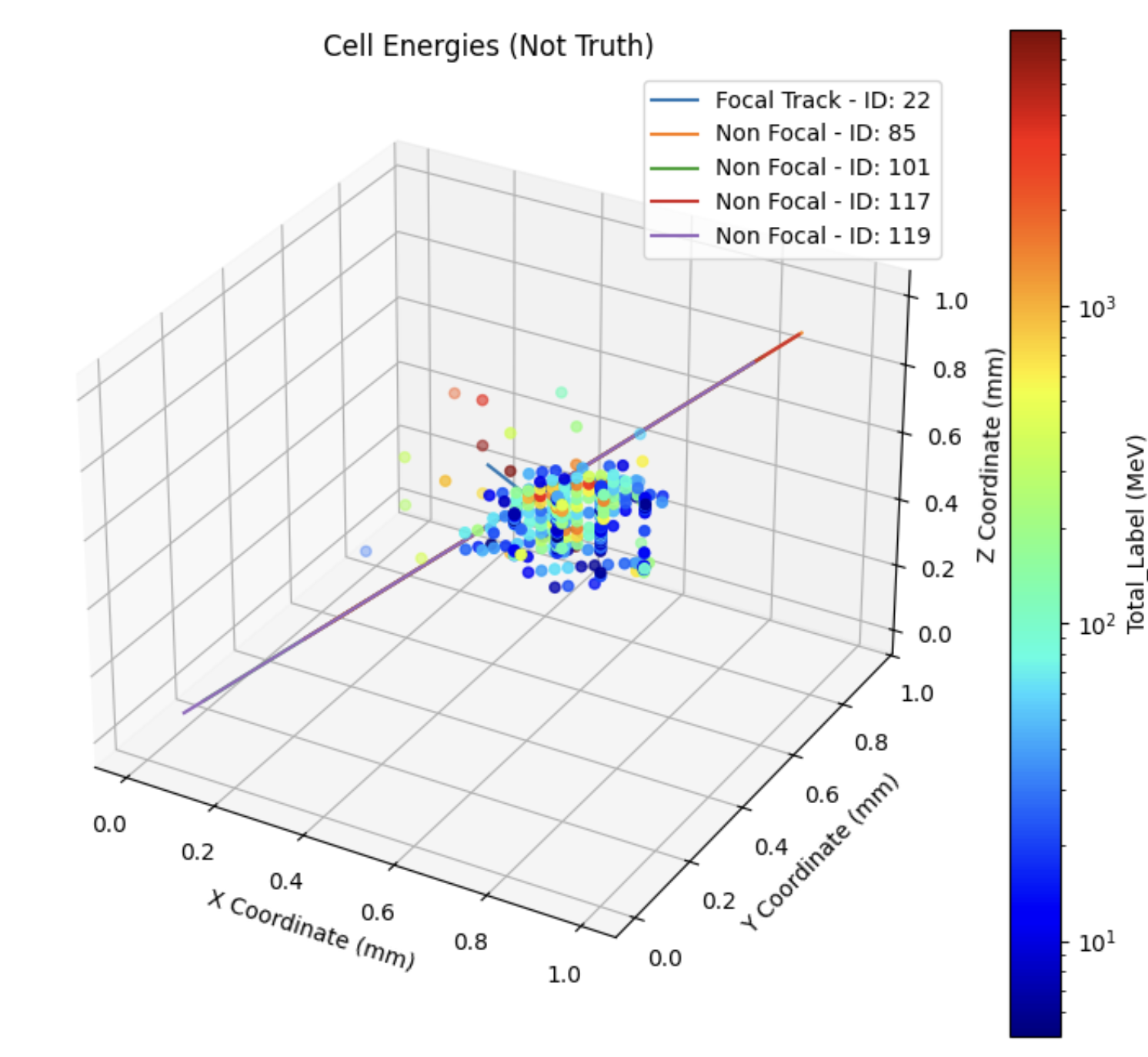
The data is represented as a point cloud where each point is a calorimeter hit. As a sparse point cloud, the data is not well suited to traditional models that rely on consistent length inputs. One approach would be to place the points into a 3D grid; however, this would be computationally expensive and require an extremely high complexity network. The solution that we are using for this problem is PointNet, a model capable of processing point clouds directly without converting them to a grid. PointNet has the advantage of being able to process clouds of arbitrary size; however, it requires several multi-layer perceptrons to provide the spatial and order invariance expected from a neural network. This idea was first introduced in the paper PointNet: Deep Learning on Point Sets for 3D Classification and Segmentation.
Data Preprocessing
One of the largest challenges of adapting the PointNet model to the ATLAS calorimeter is representing the data in a meaningful way to the model. To do this, we require several categorical inputs, including track information, calorimeter hits, and non-focal track information. While this step may seem trivial, there are several design considerations surrounding the consideration of edge cases. For instance, some tracks, when extrapolated to the calorimeter, do not intersect with any of the calorimeter layers. This is primarily observed around eta = ±2.48, where structural components of the detector prevent the track from intersecting with the calorimeter. Furthermore, the model cannot handle the immense amount of data in a single event, so each track is limited to a maximum eta-phi radius (eta-phi is a coordinate system in the calorimeter, analogous to a theta-phi system in a spherical coordinate system) to focus the model on the most relevant cells.
Furthermore, the processing time of raw data is significant, making its optimization a critical step in developing a model that could be used in a real-time setting.
Searching the Hyperparameter Space
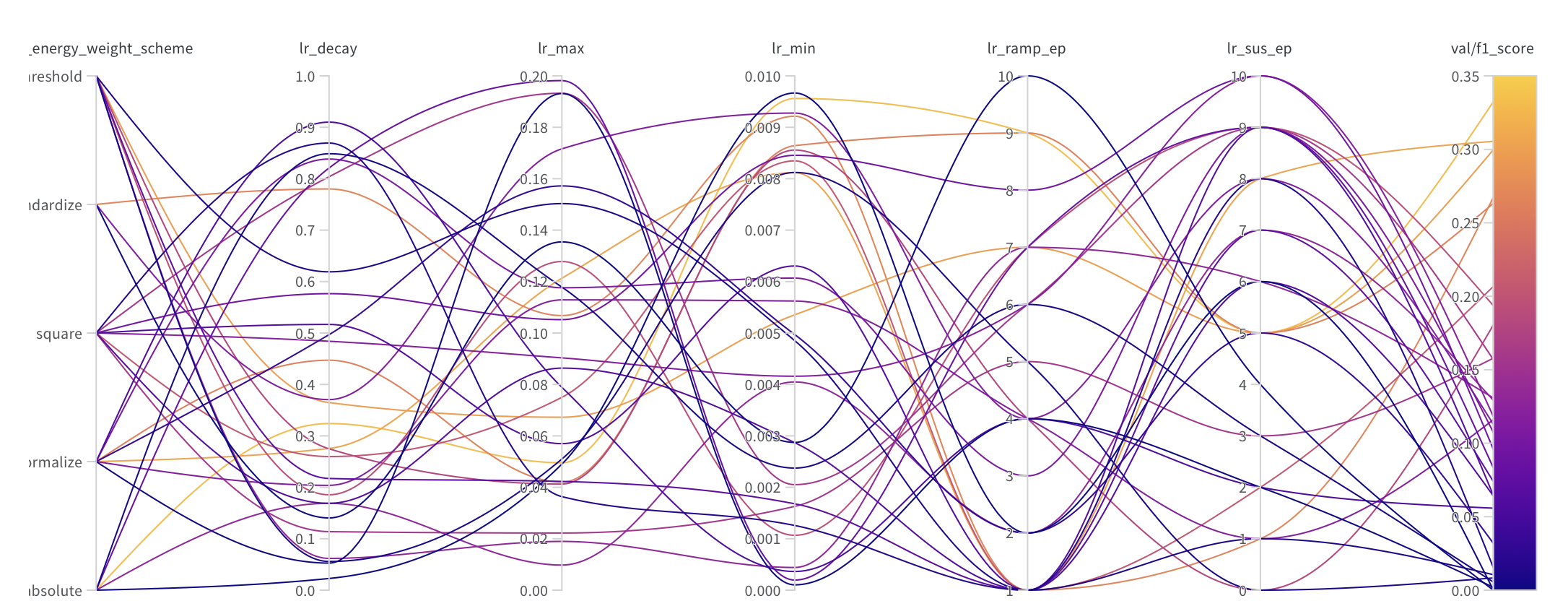
Ultimately, with a model as complex as PointNet, it is important to search the hyperparameter space to find the optimal model. It was observed that in a few cases, the model would not converge, but more importantly, the model could experience modal collapse, where the model would convert to declaring all hits as either signal or background instead of the per-hit classification that was desired. The primary mitigation against this, however, is not the hyperparameters but the data preprocessing. Particularly, expanding the training set significantly reduced the occurrence of modal collapse. The original modal collapse is believed to be a consequence of our original training on only 2000 events (~125000 tracks) with over 5 million trainable parameters. One hypothesis about why this modal collapse was so prevalent was its pure effectiveness at reducing the loss function. With a perfect model experiencing this all-on or all-off behavior, the accuracy could be as high as 87%. While technically interesting, this model is ineffective because it does not allow us to make predictions from the model outputs beyond what is already possible by applying a simple pt (momentum) cut.
For a hyperparameter search, beyond shaping the training data and model size, we completed a sweep of the phase space for the learning rate, number of epochs, and loss function energy weighting using Weights and Biases.
Choosing a Validation Metric
The model training makes use of two metrics. First, the loss function was a weighted binary cross-entropy loss function. This function was chosen because it represents the entropic relationship between the predicted and actual values, which is critical for a classification problem, as well as its differentiability, which is critical for backpropagation.
However, the relationship between the loss function and the model performance is not always clear, and the value of the loss function does not translate well to the confidence of the network. For that reason, at the hyperparameter search stage, we used the F1 score as a validation metric. F1 scores measure the model’s ability to correctly identify the signal and background events. Particularly, the F1 score is the harmonic mean of the precision and recall of the model. The F1 score is a good metric for this model because it measures the model’s ability to correctly identify signal and background events, which is the primary goal of the model. The reason that it is not used as the loss function is that it is not differentiable and therefore not suitable for backpropagation.
Results
The model is still in development and being trained on Monte Carlo data, so the results are not yet available.